
- Accessing current simulation count
- Accessing platform time and clock time
- Suppressing simulation progress
- Calculating distances between nodes
- Programmatically stopping a simulation
- Setting log level of the simulation agent
- Specifying relative paths for files
- Working with GPS coordinates
- Distributing nodes randomly
- Encoding and decoding PDUs
- Using MATLAB to plot results
- Using a visual debugger in agent development
1. Accessing current simulation count
The current simulation count can be accessed using the count variable in a simulation script. For example:
1
2
3
4
5
6
7
8
9
//! Simulation: Demo of using simulation count

[...].each { p ->
  simulate 10.hours {
    println "Simulation #${count} for parameter = ${p}"
      :
      :
  }
}
2. Accessing platform time and clock time
The platform time (discrete event or real-time) can be accessed using the time() closure in a simulation script. The clock time can be accessed using the clock() closure. Both closures provide time in seconds from some arbitrary origin. For example:
1
2
3
4
5
6
7
8
//! Simulation: Demo of clock()

def t0 = clock()
simulate 10.hours {
    :
    :
}
println "10 hours worth of simulation completed in ${clock()-t0} seconds"
3. Suppressing simulation progress
By default, the simulation progress is displayed on the terminal for Mac OS X and Linux. For Windows, due to lack of support in Cygwin for ANSI terminal sequences, this is disabled. Should you wish to suppress the display of simulation progress, set the variable showProgress in your simulation script to be false:
1
showProgress = false
4. Calculating distances between nodes
A closure distance() is available in the simulation script to compute distance between two locations:
1
2
3
def location1 = [0, 0, 0]
def location2 = [300.m, 1.km, 0]
println distance(location1, location2)
5. Programmatically stopping a simulation
You can stop a simulation from your simulation agent by calling the stop() closure. For example:
1
2
3
4
5
6
7
8
9
10
11
12
13
//! Simulation: Demo of stop()

import org.arl.fjage.TickerBehavior

simulate {
  def n = node 'AUV', address: 1
  n.startup = {
    // stop simulation with a probability of 1% at every 10 second boundary
    add new TickerBehavior(10000, {
      if (rnd(0,1) < 0.01) stop()
    })
  }
}
6. Setting log level of the simulation agent
A simple way to change log level of the simulation agent is via the logLevel variable in the simulation script. For example:
1
logLevel = java.logging.Level.ALL
7. Specifying relative paths for files
When a simulation is run, a home variable is defined to point to the simulator installation directory. This is useful to refer to common files:
1
2
// set up node 1 with stack loaded from the common setup.groovy file
node '1', address: 1, stack: "$home/etc/setup.groovy"
Another variable script is defined to point to the simulation script file being executed. This can be used to find the directory containing the script file, if other files in the same directory need to be referenced:
1
2
// load a settings file from the same directory as the script
run "${script.parent}/settings.groovy"
8. Working with GPS coordinates
Sometimes it is useful to work with GPS coordinates for node locations, but the simulator uses a local coordinate frame. Here’s how to easily convert from one to another.
First create a local coordinate system with a specified origin:
1
> gps = new org.arl.unet.utils.GpsLocalFrame(1.289545, 103.849972);
Then convert node GPS coordinates to local frame (coordinates in meters):
1
2
3
4
> gps.toLocal(1.29, 103.85)               // decimal degrees
[3.1161606856705233, 50.311549937515956]
> gps.toLocal(1, 17.4, 103, 51)           // degrees, decimal minutes
[3.1161606856705233, 50.311549937515956]
or convert from local frame to GPS coordinates:
1
2
3
4
> gps.toGps(1000.m, 500.m)                // decimal degrees
[1.2940668245170857, 103.85895741597328]
> gps.toGpsDM(1000.m, 500.m)              // degrees, decimal minutes
[1.0, 17.64400947102514, 103.0, 51.53744495839675]
There are other options for GPS coordinate formats too (e.g. degrees, minutes, seconds).
9. Distributing nodes randomly
Often, in simulations, we wish to distribute nodes randomly in a given area. Here’s how to do that in a simulation script:
1
2
3
4
5
6
7
8
9
10
11
12
13
14
//! Simulation: Demo of randomly deployed nodes

platform = org.arl.fjage.RealTimePlatform

def n = 10          // number of nodes
def xsize = 1.km    // distribute nodes in a 1.km x 1.km box, within a depth of 20.m
def ysize = 1.km
def maxdepth = 20.m

simulate {
  n.times {
    node "${it+1}", location: [rnd(-xsize/2, xsize/2), rnd(-ysize/2, ysize/2), rnd(-maxdepth, 0)]
  }
}
10. Encoding and decoding PDUs
When implementing protocols, we often need to assemble and parse PDUs. To ease this task, we have a PDU utility class to help. We first define a class with our PDU format:
1
2
3
4
5
6
7
8
9
10
11
12
13
14
 import java.nio.ByteOrder
 import org.arl.unet.PDU

 class MyPDU extends PDU {
   void format() {
     length(16)                     // 16 byte PDU
     order(ByteOrder.BIG_ENDIAN)    // byte ordering is big endian
     uint8('type')                  // 1 byte field 'type'
     uint8(0x01)                    // literal byte 0x01
     filler(2)                      // 2 filler bytes
     uint16('data')                 // 2 byte field 'data' as unsigned short
     padding(0xff)                  // padded with 0xff to make 16 bytes
   }
}
We can then encode and decode PDUs easily using this class:
1
2
3
4
5
> pdu = new MyPDU();
> bytes = pdu.encode([type: 7, data: 42])
[7, 1, 0, 0, 0, 42, -1, -1, -1, -1, -1, -1, -1, -1, -1, -1]
> pdu.decode(bytes)
[data:42, type:7]
In some cases, it is convenient to define a PDU without explicitly defining a new class. In that case, we can create an anonymous class with the standard Java syntax, or using the Groovy extensions syntax shown here:
1
2
3
4
5
6
7
8
9
10
11
def pdu = PDU.withFormat {
  length(16)                     // 16 byte PDU
  order(ByteOrder.BIG_ENDIAN)    // byte ordering is big endian
  uint8('type')                  // 1 byte field 'type'
  uint8(0x01)                    // literal byte 0x01
  filler(2)                      // 2 filler bytes
  uint16('data')                 // 2 byte field 'data' as unsigned short
  padding(0xff)                  // padded with 0xff to make 16 bytes
}
bytes = pdu.encode([type: 7, data: 42])
data = pdu.decode(bytes)
For further information, see PDU API documentation.
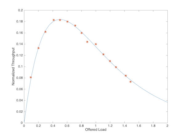
11. Using MATLAB to plot results
The samples provided with UnetStack show how to plot results (e.g. samples/aloha/plot-results.groovy) using a Groovy script. Sometimes you may wish to use other tools such as MATLAB to analyze the results. To do this, you’ll need to extract relevant results from the log file and then load them in MATLAB.
For example, let us assume that you just ran the samples/aloha/aloha.groovy simulation and have the log files in the logs directory. You can extract the relevant STATS lines from the log file and reformat into a CSV file that MATLAB can load:
1
bash$ grep STATS logs/trace.nam | sed 's/.=//g' | sed 's/^# STATS: //' > logs/results.txt
Then open MATLAB and load the data in MATLAB, and plot it:
1
2
3
4
5
6
7
8
>> load logs/results.txt
>> x = 0:0.05:2;
>> plot(x, x.*exp(-2*x))
>> hold all
>> plot(results(:,5),results(:,8),'*')
>> hold off
>> ylabel('Normalized Throughput');
>> xlabel('Offered Load');
The output should look like this:
12. Using a visual debugger in agent development
While the Unet Simulator does not have an integrated debugger, it is possible to use a debugger from another IDE (e.g. IntelliJ IDEA or Eclipse) with UnetStack. The basic steps are outlined below, but the exact details depend on the IDE used:
- Downloaded and install the IDE with Groovy support.
- Create a Groovy project and add all UnetStack jars as external libraries. You should find the jars in the
libfolder. - Create a configuration with main class org.arl.fjage.shell.GroovyBoot and arguments cls://org.arl.unet.sim.initrc followed by the simulation script filename.
- Start a debugging session. More details for using IntelliJ IDEA can be found here.