
A common problem in mobile robotics deals with answering the question: “Where am I?”. If the robot is equipped with GPS (Global Positioning System) receiver, it can be localized accurately. Unfortunately, GPS doesn’t work underwater. For GPS to work underwater, the GPS receiver should be able to receive the Radio Frequency (RF) signals from GPS satellites. But RF signals do not propagate well in water and therefore GPS receiver cannot receive the signals underwater. Acoustic communication is the most promising mode of communication underwater. With static reference underwater acoustic modems acting as “satellites” in the ocean, we can localize an underwater robot/vehicle.
The objective of this blog is to present the solution for this problem considering a simple scenario and demonstrate the simple steps in which localization algorithm can be implemented. For the purpose of this blog, we will use UnetStack (an underwater network stack and simulator).
Objective
Simply put, the following is our objective:
Given two landmarks at which the underwater acoustic modems are deployed and their locations in Cartesian space is known, and an underwater static or mobile node (e.g. an AUV, underwater robot etc.) equipped with an underwater acoustic modem, the task is to determine the AUV’s location in Cartesian space.
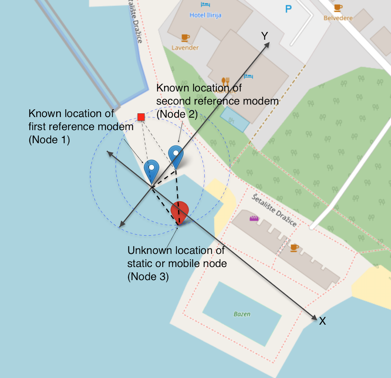
The figure shown above illustrates the setup that is considered. The blue markers are the landmarks with the known locations where the modems are deployed. These locations can be GPS coordinates at the point of deployment. The red markers show where the unknown location of the target node could be. We refer the node which needs to be localized as the target node. The origin is set at Node 1 and the XY plane is visualized as shown in the figure above.
Note that at least three reference nodes/modems are required to uniquely localize the coordinates in the XY plane. Since in this case, we have only two modems (Node 1 and Node 2) acting as the reference nodes, there will be an ambiguity in the location of Node 3 when trying to localize. A convenient assumption we make here is that the target node (Node 3) is only deployed in the right side of the origin (i.e., the abscissa is positive).
The GPS coordinates at these known locations are converted to local cartesian coordinates. Let the GPS locations at which the modems are deployed be:
Node 1 –> (43.933777, 15.443508) –> Origin
Node 2 –> (43.933901, 15.443539)
Node 3 –> Target node which needs to be localized
At this point, a natural question that arises is how to convert the GPS coordinates to local coordinates.
Using Location agent in UnetStack
UnetStack comes equipped with NodeInfo agent and NODE_INFO service that will keep track of the modem location (as well as other parameters like speed, heading etc.), which can be used to geotag individual transmissions or receptions. A simple Unet agent that will update the location parameter of the node agent, in a periodic manner using the GPS data stream from a GPS server running on terrestrial network is available as part of UnetStack as Location agent. The interested reader may find this blog on developing Location agent useful for more details. The Location agent converts the GPS coordinates to local coordinate system and maintains it in the location parameter of the NodeInfo agent.
Open connection to the modem or real-time simulator
For the purpose of illustration, we deploy a 3-node network in Unet simulator as per the locations in the above-shown figure. We connect to the Node 1 running on localhost port 1101 and Node 2 running on localhost port 1102.
1
2
3
4
5
6
7
from unetpy import *

node1gw = UnetGateway('localhost', 1101)
node1 = node1gw.agentForService(Services.NODE_INFO)

node2gw = UnetGateway('localhost', 1102)
node2 = node2gw.agentForService(Services.NODE_INFO)
If we are connected to the modem, we can now access the agents and services that the modem provides. Let us try this with the NodeInfo agent. What you’ll see here depends on the network that is deployed in the simulator.
1
print(node1)
1
2
3
4
5
6
7
8
9
10
11
12
[org.arl.unet.nodeinfo.NodeInfoParam]
  address = 1
  canForward = False
  diveRate = 0.0
  heading = 0.0
  location = [0.0, 0.0, 0.0]
  mobility = False
  nodeName = 1
  origin = []
  speed = 0.0
  time = Sep 24, 2018 2:02:23 PM
  turnRate = 0.0
1
print(node2)
1
2
3
4
5
6
7
8
9
10
11
12
[org.arl.unet.nodeinfo.NodeInfoParam]
  address = 2
  canForward = False
  diveRate = 0.0
  heading = 0.0
  location = [2.4141898796660826, 13.78562671598047, 0.0]
  mobility = False
  nodeName = 2
  origin = []
  speed = 0.0
  time = Sep 24, 2018 2:02:23 PM
  turnRate = 0.0
The above presents the NodeInfo parameters for the specific nodes, Node 1 and Node 2. These parameters can be useful in the localization application, where the location of a mobile node keeps getting updated and needs to be maintained. The location of Node 1 and Node 2 in the above simulation is shown by the Cartesian coordinates in meters.
Ranging to measure distances
Now, that the network simulator is set up with two known locations of the modem in the local coordinates system, we set out to compute the GPS location of the third node. We need to measure the distance from the two known locations to the modem we are trying to locate. This can be achieved using ranging functionality in UnetStack.
1
2
3
4
5
ranging_node1 = node1gw.agentForService(Services.RANGING)
node1gw.subscribe(ranging_node1)
ranging_node1 << org_arl_unet_phy.RangeReq(to=3)
rnf1 = node1gw.receive(RangeNtf, 5000)
range1 = rnf1.getRange()
1
2
3
4
5
ranging_node2 = node2gw.agentForService(Services.RANGING)
node2gw.subscribe(ranging_node2)
ranging_node2 << org_arl_unet_phy.RangeReq(to=3)
rnf2 = node2gw.receive(RangeNtf, 5000)
range2 = rnf2.getRange()
The distances are measured using acoustic ranging as shown above and stored in variables range1 and range2.
Localization algorithm
There are more than one way to compute the location of the third node. We present below two methods:
-
Minimization of squared error
-
Geometric circle intersection
Although, we prefer the first method since it can be easily scaled when there are more number of reference nodes with known locations are available.
Minimization of squared error
Let the local coordinates of the target node be denoted by a vector \(\mathbf{x}\) and the known positions of the \(i^{\text{th}}\) reference node be denoted by vector \(\mathbf{p}_i\). The range measured from the \(i^{\text{th}}\) reference node to the target node is denoted by \(r_i\).
Now, we can formulate an optimization objective to minimize the sum of squared error and try to estimate an optimal value of \(\mathbf{x}\). The problem is formulated as shown below:
\[\mathbf{x}^* = \arg\min_\mathbf{x} \sum_i \left(\left|\;\mathbf{x}-\mathbf{p}_i\;\right|-r_i\right)^2\]The above problem can be implemented in python and solved using using methods in scipy module as shown below;
1
2
3
4
5
6
7
8
9
10
11
12
import math
from scipy.optimize import minimize

def norm(x):
    return math.sqrt(np.sum(x**2))

def cost(x):
    loc = np.asarray(locations)
    return (norm(x-loc[0])-range1)**2 + (norm(x-loc[1])-range2)**2

soln = minimize(cost, (-10,20))
print(list(soln.x))
1
[-19.608792834527456, 6.4265057515711765]
The above shown is the local coordinate found by solving the optimization problem. Next we will compare this solution with the geometric circle intersention method and finally update this computed location on the map.
Geometric circle intersection method
The Geometric circle intersection method is widely used in literature. Conceptually, the idea is straightforward. Referring to the figure above, there are two circles that can be formed with the reference modems at the center. There are only two possible location where these circles can intersect. As noted before, a third reference modem can remove this ambiguity, however, in the absence of the third reference modem, the two possible locations are shown with red marker in the figure at the two intersection points of the circle. With the assumption that the unknown node is deployed only on one side of the XY plane, the position of the target node can be computed uniquely.
Let us denote the unknown/target node’s (Node 3) location be \((x_1, x_2)\).
The known positions of the Node 1 is denoted by \((a_1, a_2)\) and Node 2 by \((b_1, b_2)\).
The measured distances to Node 3 from Node 1 and Node 2 are denoted by \(r_1\) and \(r_2\) respectively.
Given the above information, two seconnd order equations in two variables \(x_1\) and \(x_2\) can be written as follows:
\[(x_1-a_1)^2 + (x_2-a_2)^2 - r_1^2 = 0\]and
\[(x_1-b_1)^2 + (x_2-b_2)^2 - r_2^2 = 0\]We use the symbolic manipulation toolbox sympy in python to compute the analytic expression for computing \((x_1, x_2)\). The details are as given below:
1
from sympy import *
1
x1, x2, a1, a2, b1, b2, r1, r2 = symbols('x1 x2 a1 a2 b1 b2 r1 r2')
Write the variable \(x_1\) in terms of all other known parameters and variable \(x_2\)
1
x1 = ((a1**2 - b1**2) + (a2**2 - b2**2) - (r1**2 - r2**2) -2*x2*(a2-b2))/(2*(a1-b1))
Compute the expression for \(x_2\) symbolically
1
expr = solveset(Eq((x1 - a1)**2 + (x2 - a2)**2 - r1**2, 0), x2)
Now we know the expression for \(x_2\) in terms of all known parameters. Therefore, it’s value can be computed using substitution as shown below:
1
2
3
x2_sol = list(expr.subs([(a1, node1.location[0]), (a2, node1.location[1]), \
           (b1, node2.location[0]), (b2, node2.location[1]), \
           (r1, range1), (r2, range2)]).evalf())
There are two possible solutions. The decision is based on the value of \(x_1\), since our modem which is being localized lies on the right side of the y-axis, we take the decision based on the sign of \(x_1\).
1
x2_sol
1
[6.4265057515711765, 30.1984110020781]
The value of \(x_1\) is computed for both values of computed \(x_2\).
1
2
3
4
5
6
7
8
9
x1_sol = []
x1_sol.append( x1.subs([(a1, node1.location[0]), (a2, node1.location[1]), \
               (b1, node2.location[0]), (b2, node2.location[1]), \
               (r1, range1), (r2, range2), \
               (x2, x2_sol[0])]).evalf() )
x1_sol.append( x1.subs([(a1, node1.location[0]), (a2, node1.location[1]), \
               (b1, node2.location[0]), (b2, node2.location[1]), \
               (r1, range1), (r2, range2), \
               (x2, x2_sol[1])]).evalf() )
1
x1_sol
1
[-19.608792834527456, -15.2487662763113]
1
2
3
4
index = [idx for idx, val in enumerate(x1_sol) if val >= 0][0]
x1 = x1_sol[index]
x2 = x2_sol[index]
print((x1, x2, 0.0))
1
(-19.608792834527456, 6.4265057515711765, 0.0)
Update the map with the computed location
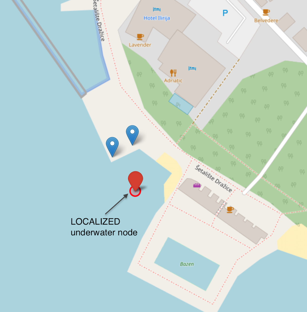
The map is updated with the localized node’s location with a red circle as shown in the figure above. In conclusion, we saw how easily such a localization application can be developed utilizing UnetStack.
For interested reader, the jupyter notebook with the complete code in Python can be found at this link.